8 付録: 記述統計

関心のあるグループ \((D)\) ごとに記述統計をまとめる
Section 8.2 記述統計表を作成
Section 8.3 ヒストグラムを用いた比較
Section 8.4 変数の分布がバランスしているかどうか、図示する

8.1 設定

R
Python

library(tidyverse)
library(gtsummary) # 記述統計
library(cobalt) # バランス確認

Data_R <- read_csv("ExampleData/Example.csv")

gtsummary : 記述統計表作成
cobalt : 図作成

import pandas as pd
import seaborn as sns # 可視化


Data_Python = pd.read_csv('ExampleData/Example.csv')

8.2 記述統計表

\(D=Reform\) ごとに以下を表示

R
Python

連続変数については、 “中央値(下位25%, 上位25%)”
カテゴリー変数について、 “サンプルサイズ(割合)”

Data_R |> 
  tbl_summary(by = "Reform")

Characteristic	0, N = 11,012¹	1, N = 3,781¹
TradeQ
1	2,864 (26%)	963 (25%)
2	2,940 (27%)	967 (26%)
3	2,682 (24%)	914 (24%)
4	2,526 (23%)	937 (25%)
Size	45 (25, 65)	50 (35, 65)
BuildYear	2,006 (1,998, 2,012)	1,995 (1,984, 2,003)
Distance	6.0 (4.0, 9.0)	7.0 (4.0, 10.0)
Price	31 (22, 50)	34 (24, 48)
¹ n (%); Median (IQR)

Data_Python.groupby('Reform').describe().T

Reform                      0            1
TradeQ    count  11012.000000  3781.000000
          mean       2.442245     2.482677
          std        1.107117     1.120293
          min        1.000000     1.000000
          25%        1.000000     1.000000
          50%        2.000000     2.000000
          75%        3.000000     3.000000
          max        4.000000     4.000000
Size      count  11012.000000  3781.000000
          mean      45.175490    49.809574
          std       22.727207    20.268129
          min       10.000000    10.000000
          25%       25.000000    35.000000
          50%       45.000000    50.000000
          75%       65.000000    65.000000
          max      125.000000   125.000000
BuildYear count  11012.000000  3781.000000
          mean    2003.263187  1993.545579
          std       12.008525    12.893772
          min     1963.000000  1964.000000
          25%     1998.000000  1984.000000
          50%     2006.000000  1995.000000
          75%     2012.000000  2003.000000
          max     2022.000000  2021.000000
Distance  count  11012.000000  3781.000000
          mean       6.973628     7.275513
          std        4.049774     4.109578
          min        0.000000     0.000000
          25%        4.000000     4.000000
          50%        6.000000     7.000000
          75%        9.000000    10.000000
          max       22.000000    21.000000
Price     count  11012.000000  3781.000000
          mean      39.529176    40.086363
          std       32.085602    27.362758
          min        0.500000     0.540000
          25%       22.000000    24.000000
          50%       31.000000    34.000000
          75%       50.000000    48.000000
          max     1600.000000   300.000000

8.3 ヒストグラム

\(D=Reform\) ごとに以下を表示

R
Python

Data_R |> 
  mutate(Reform = factor(Reform)) |> 
  ggplot(
    aes(
      x = Size,
      fill = Reform,
      group = Reform
      )
    ) +
  geom_histogram(
    aes(y=..density..),
    alpha=0.5,
    position='identity'
    ) +
  theme_bw()

sns.displot(
  Data_Python, 
  x="Size", 
  hue="Reform", 
  stat="density",
  common_norm=False)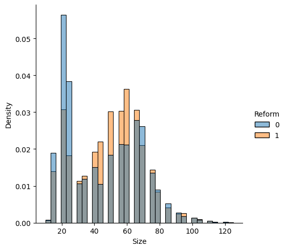

8.4 バランス確認

異なるDグループ間で、Xの分布の違いを確認
Xの平均差/Xの標準偏差を報告 (Imbens (2015) などで推奨)

R
Python

bal.tab(Reform ~ Size + BuildYear + Distance + TradeQ,
        Data_R,
        binary = "std", continuous = "std") |> 
  plot()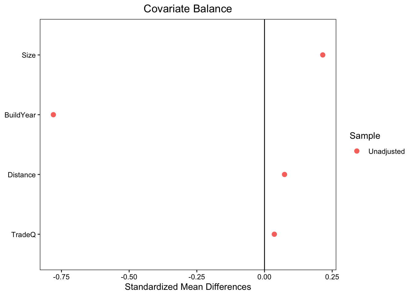

築年が古い、広い、駅からの距離が長い物件が、改装されがち

Under construction