5  直接的なBalancing Weightの算出

Hainmueller (2012) や Zubizarreta (2015) では、Balancing Weightを明示的な”最小化問題”の解として算出します。 このようなアプローチは、満たすべき条件(負の荷重が生じない/サンプル平均にバランスするなど）を課した上で、Balancing Weightが算出できます。 このためOLSによる暗黙のBalancingに比べて、より透明性の高い分析が可能です。

5.1 算出方法

Balancing Weightについて、以下のような制約を課します。

1. 全ての\(X_l\)について、その加重平均をデータ全体の平均値に一致させる: \[(D=1)における(\omega(x,1)\times X_l)の平均値\] \[= (D=0)における(\omega(x,0)\times X_l)の平均値\] \[= X_lのデータ全体での平均値\]

2. 全てのWeightは非負の値をとる: \[\omega(x,d)\ge 0\]

上記の制約を満たす\(\omega(d,x)\) のなかで、最もばらつきが小さいものをBalancing Weightとします。 ばらつきの測定方法は、いくつかの提案があります。

• Hainmueller (2012) : \(\omega(x,d)\) のentropy divergence \(\omega(x,d)\log(\omega(x,d)/q)\)

  • \(q\) はbase weightと呼ばれ、例えば \(q=1/事例数\) が用いられます。

• Zubizarreta (2015) : \(\omega(x,d)\) の分散

特にentropy divergenceを用いる Hainmueller (2012) の方法は、実際の計算も早く実用的です。 以下では、実際の実装方法を紹介します。

5.2 Rによる実践例

• \(D\)と\(X\)の交差項を含めたモデルのOLS推定、およびその性質の診断は、以下のパッケージを用いて実装できます。

  • readr (tidyverseに同梱): データの読み込み

  • WeightIt: entroy weightの計算

    • Repository

  • marginaleffects: WeightItパッケージが計算するWeightを用いた推定

    • Repository

5.2.1 準備

データを取得します。 \(D\) として、立地が中心6区か否かで、1/0となる変数を定義します。

Data = readr::read_csv("Public.csv") # データ読み込み

Data = dplyr::mutate(
  Data,
  D = dplyr::if_else(
    LargeDistrict == "中心6区",1,0
  ) # 中心6区に立地していれば1、それ以外は0
)

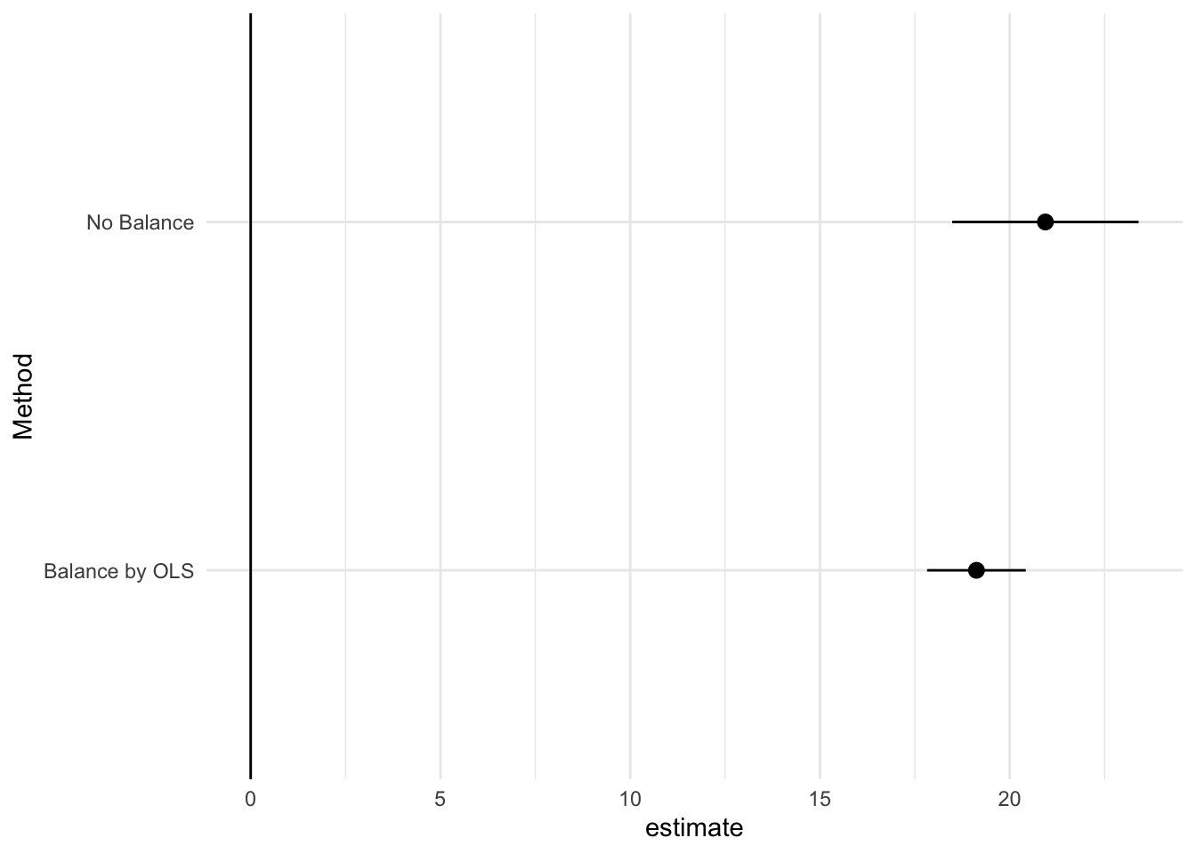
ベンチマークとして、一切のバランスを行わない単純差、およびOLSによるバランスを行った結果を示します。

Model_No = estimatr::lm_robust(Price ~ D, Data)

Model_OLS = estimatr::lm_robust(
  Price ~ D + (Size + Tenure + StationDistance)**2 +
    I(Size^2) + I(Tenure^2) + I(StationDistance^2), 
  Data)

Model_No |> 
  generics::tidy() |> 
  dplyr::mutate(
    Method = "No Balance"
  ) |> 
  dplyr::bind_rows(
    Model_OLS |> 
  generics::tidy() |> 
  dplyr::mutate(
    Method = "Balance by OLS"
  )
  ) |> 
  dplyr::filter(
    term == "D"
  ) |> 
  ggplot2::ggplot(
    ggplot2::aes(
      y = Method,
      x = estimate,
      xmin = conf.low,
      xmax = conf.high
    )
  ) +
  ggplot2::geom_pointrange() +
  ggplot2::theme_minimal() +
  ggplot2::geom_vline(
    xintercept = 0
  )

5.2.2 Entropy Weightによるバランス

\(D\) 間でSize,Tenure,StationDistanceの平均値をバランスさせ、Priceの平均値を比較します。 まずWeightItパッケージを用いて、Entropy Weightを計算します。 また比較のためにlmwパッケージを用いて、OLS Weightも計算します。

Entropy = WeightIt::weightit(
  D ~ (Size + Tenure + StationDistance)**2 +
    I(Size^2) + I(Tenure^2) + I(StationDistance^2),  # 平均、分散、共分散をバランス
  data = Data,
  method = "ebal", # Entropy Weightを計算
  estimand = "ATE") 

OLS = lmw::lmw(
  ~ D + (Size + Tenure + StationDistance)**2 +
    I(Size^2) + I(Tenure^2) + I(StationDistance^2),
  Data
)

summary関数を用いて、Weightの分布を確認します。

summary(Entropy$weights)

   Min. 1st Qu.  Median    Mean 3rd Qu.    Max. 
 0.2533  0.8622  0.9706  1.0000  1.0877 16.5677 

summary(OLS$weights)

   Min. 1st Qu.  Median    Mean 3rd Qu.    Max. 
-0.2343  0.7615  1.0007  1.0000  1.2484  2.7393 

OLSを用いると負のBalancing weightが発生していることが確認できます。 対してEntropy weightでは、そのようなweightは生じません。

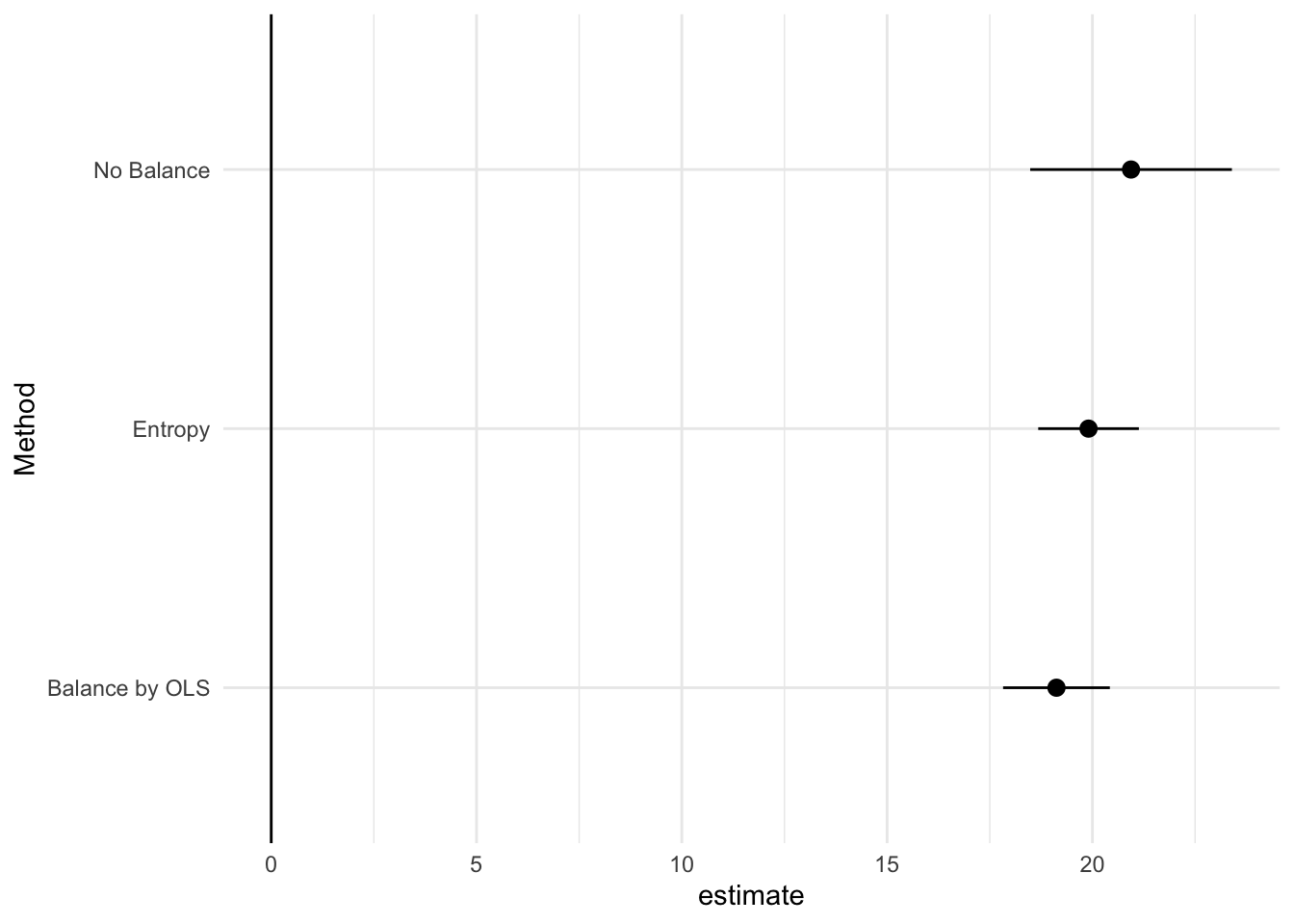
Entropy Weightを用いたバランス後の平均差は、marginaleffectsパッケージのavg_comparison関数を用いて、以下のように計算できます。

WeightIt::lm_weightit(
  Price ~ D*(I(Size^2) + I(Tenure^2) + I(StationDistance^2) +
    (Size + Tenure + StationDistance)**2),
  data = Data,
  weightit = Entropy
  ) |> 
  marginaleffects::avg_comparisons(variables = "D")

 Estimate Std. Error    z Pr(>|z|)     S 2.5 % 97.5 %
     19.9      0.625 31.8   <0.001 736.2  18.7   21.1

Term: D
Type:  probs 
Comparison: 1 - 0

引き続き20前後の平均価格差が算出されました。

最後にバランスなし、OLSによるバランス、Entropy Weightによるバランス、の結果を図示します。

Model_Ent = WeightIt::lm_weightit(
  Price ~ D*(I(Size^2) + I(Tenure^2) + I(StationDistance^2) +
    (Size + Tenure + StationDistance)**2),
  data = Data,
  weightit = Entropy
  ) |> 
  marginaleffects::avg_comparisons(variables = "D")


Model_No |> 
  generics::tidy() |> 
  dplyr::mutate(
    Method = "No Balance"
  ) |> 
  dplyr::bind_rows(
    Model_OLS |> 
  generics::tidy() |> 
  dplyr::mutate(
    Method = "Balance by OLS"
  )
  ) |> 
  dplyr::filter(
    term == "D"
  )|> 
  dplyr::bind_rows(
    tibble::tibble(
      Method = "Entropy",
      estimate = Model_Ent$estimate,
      conf.low = Model_Ent$conf.low,
      conf.high = Model_Ent$conf.high
    )
  ) |> 
  ggplot2::ggplot(
    ggplot2::aes(
      y = Method,
      x = estimate,
      xmin = conf.low,
      xmax = conf.high
    )
  ) +
  ggplot2::geom_pointrange() +
  ggplot2::theme_minimal() +
  ggplot2::geom_vline(
    xintercept = 0
  )

5.3 発展

Balancing Weightを直接算出する方法は、近年改めて注目を集めており、さまざまな提案がなされています。 例えばAuto debiased machine learning (Chernozhukov, Newey, and Singh 2022a, 2022b; Chernozhukov et al. 2022) と呼ばれる手法も、分布をバランスするWeightを機械学習などを用いて直接算出する手法であるとの解釈も提案されています (Bruns-Smith et al. 2023) 。 Energy Weight (Huling and Mak 2024) も、特徴ではなく分布そのものをバランスするWeightの推定を行なっています。

直接計算する手法は、AIPWなどの間接的な方法 (Chapter 7) に比べて、推定結果が安定しやすいことが利点として挙げられます。

Bruns-Smith, David, Oliver Dukes, Avi Feller, and Elizabeth L Ogburn. 2023. “Augmented Balancing Weights as Linear Regression.” arXiv Preprint arXiv:2304.14545.

Chernozhukov, Victor, Whitney K Newey, and Rahul Singh. 2022a. “Automatic Debiased Machine Learning of Causal and Structural Effects.” Econometrica 90 (3): 967–1027.

———. 2022b. “Debiased Machine Learning of Global and Local Parameters Using Regularized Riesz Representers.” The Econometrics Journal 25 (3): 576–601.

Chernozhukov, Victor, Whitney Newey, Vıctor M Quintas-Martınez, and Vasilis Syrgkanis. 2022. “Riesznet and Forestriesz: Automatic Debiased Machine Learning with Neural Nets and Random Forests.” In International Conference on Machine Learning, 3901–14. PMLR.

Hainmueller, Jens. 2012. “Entropy Balancing for Causal Effects: A Multivariate Reweighting Method to Produce Balanced Samples in Observational Studies.” Political Analysis 20 (1): 25–46.

Huling, Jared D, and Simon Mak. 2024. “Energy Balancing of Covariate Distributions.” Journal of Causal Inference 12 (1): 20220029.

Zubizarreta, José R. 2015. “Stable Weights That Balance Covariates for Estimation with Incomplete Outcome Data.” Journal of the American Statistical Association 110 (511): 910–22.