Chapter 5 条件付き平均効果関数の推定

5.1 問題設定

条件付き平均差関数 \(\tau(d,d',x)=E[Y_i|D_i=d,X_i=x]-E[Y_i|D_i=d',X_i=x]\) を推定
大きく２種類の推定戦略を紹介

パラメトリック な近似モデル: \(\tau(d,d',z)\) の有限のパラメータからなる近似モデルを推定

前章の周辺化平均もこの一種: \(\tau(d,d',x) \approx \beta\) として近似
線形モデル \(\tau(d,d',x) \approx \beta_0 + \beta_1X_1+...+\beta_LX_L\) で近似
どちらの場合であっても信頼区間を計算可能

ノンパラメトリック モデル: 教師付き学習によりノンパラメトリックに推定

一般に信頼区間の計算が困難
Causal Forest algorismは例外的に漸近正規性に基づく信頼区間の近似計算を提供

5.2 パッケージ

library(tidyverse)
library(AER)
library(recipes)
library(grf)
library(rpart)
library(rpart.plot)

5.3 データ

data("PSID1982")

set.seed(123)

Y <- PSID1982$wage |> log() # 結果変数

D <- if_else(PSID1982$occupation == "white",1,0)

X <- recipe(~ education + south + smsa + gender + ethnicity + industry + weeks,
            PSID1982) |> 
  step_other(all_nominal_predictors(),
             other = "others") |> 
  step_unknown(all_nominal_predictors()) |> 
  step_indicate_na(all_numeric_predictors()) |> 
  step_impute_median(all_numeric_predictors()) |> 
  step_dummy(all_nominal_predictors()) |> 
  step_zv(all_numeric_predictors()) |> 
  prep() |> 
  bake(PSID1982)

X <- as.matrix(X)

set.seed(123)

5.4 Casual Forest

Causal Forest (Wager and Athey 2018; Athey et al. 2019) を基盤とした推定方法を紹介
- \(\tau(X)\) は以下の一般化された部分線形モデルで定義

\[E[Y|D,X]=\tau(X)\times D + f(X)\]

Random Forest をベースに \(\tau(X)\) の近似関数を推定

fit <- regression_forest(X = X,
                         Y = Y)

Y.hat <- predict(fit)$predictions

fit <- regression_forest(X = X,
                         Y = D)

D.hat <- predict(fit)$predictions


fit.CF <- causal_forest(X = X,
                        W = D,
                        Y = Y,
                        Y.hat = Y.hat,
                        W.hat = D.hat,
                        num.trees = 4000
                        )

5.5 Best linear predictors

線形近似モデル \(\tau(x)\approx \beta_0 + \beta_1X_1+...+\beta_LX_L\) を推定
\(X\) はscale関数によって標準化
- \(\beta_0\) を”平均効果”として解釈可能

best_linear_projection(fit.CF,scale(X))

## 
## Best linear projection of the conditional average treatment effect.
## Confidence intervals are cluster- and heteroskedasticity-robust (HC3):
## 
##                   Estimate  Std. Error t value Pr(>|t|)   
## (Intercept)     0.19596292  0.07019857  2.7916 0.005416 **
## education       0.08618803  0.07001161  1.2311 0.218796   
## weeks           0.06479440  0.05452998  1.1882 0.235222   
## south_yes      -0.05390008  0.05280003 -1.0208 0.307753   
## smsa_yes       -0.06226340  0.06482436 -0.9605 0.337202   
## gender_female   0.00019173  0.03808792  0.0050 0.995985   
## ethnicity_afam -0.06304902  0.04463958 -1.4124 0.158362   
## industry_yes   -0.07646084  0.06049545 -1.2639 0.206764   
## ---
## Signif. codes:  0 '***' 0.001 '**' 0.01 '*' 0.05 '.' 0.1 ' ' 1

5.6 Distribution of predicted individual effects

一般にノンパラメトリック モデルでは、信頼区間計算が難しい
- \(X\) の数が少ないCausal forestでは “例外”的に計算可能

df <- mutate(PSID1982,
             tau = predict(fit.CF,
                               estimate.variance = TRUE)$predictions,
             sd = predict(fit.CF,
                               estimate.variance = TRUE)$variance.estimates |> sqrt())

df |> 
  arrange(tau) |> 
  ggplot(aes(x = c(1:nrow(df)),
             y = tau,
             ymin = tau - 1.96*sd,
             ymax = tau + 1.96*sd)
         ) +
  geom_ribbon(alpha = 0.8) +
  geom_line() +
  geom_hline(yintercept = 0) +
  theme_bw()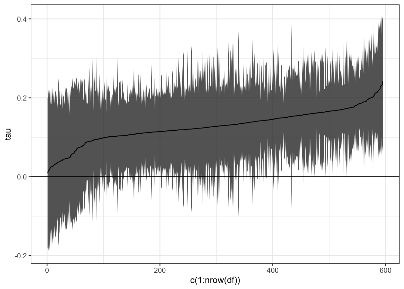

References

Athey, Susan, Julie Tibshirani, Stefan Wager, et al. 2019. “Generalized Random Forests.” Annals of Statistics 47 (2): 1148–78.

Wager, Stefan, and Susan Athey. 2018. “Estimation and Inference of Heterogeneous Treatment Effects Using Random Forests.” Journal of the American Statistical Association 113 (523): 1228–42.