Chapter 6 Panel data
\(\{Y_{it},D_{it},X_{it}\}\)が観察できるデータを想定する
- \(i:\)回答者、\(t:\)回答時点
6.1 パッケージ
library(tidyverse)
library(estimatr)
library(AER)
library(did) # weighted two-way fixed effect
6.2 Data
AERパッケージに含まれるパネルデータPSID7682を利用
- 595名の回答者について、1976年から1983年までの7期間パネルデータ
data("PSID7682")

data <-
  PSID7682 |>
  group_by(id) |>
  mutate(period = as.numeric(year), # yearを連続変数化
         treatment.time = if_else(married == "yes",
                                  period,
                                  999),
         treatment.time = min(treatment.time)
         ) |>  # 結婚したperiodを作成(結婚しなかったサンプル = 9999)
  ungroup()
6.3 識別: Pallarel trend in the two-by-two case
2時点・2グループデータ
トリートメントグループ: 2期目に介入を受ける
コントロールグループ: 両期間ともに介入を受けない
Pallalel trendの仮定 \(E[Y_{2i}(0)-Y_{1i}(0)|i\in Treatment]-E[Y_{2i}(0)-Y_{1i}(0)|i\in Control]\)
差の差の推定量を推定
\[E[Y_{i2}|i\in Treatment]-E[Y_{i1}|i \in Treatment]\]
\[-(E[Y_{i2}|i\in Control]-E[Y_{i1}|i \in Control])\]
\[= E[Y_{i2}(1) - Y_{i2}(0)|i \in Treatment]\]
6.4 推定: Two-way fixed effect model
- Two-way fixed effect model
\[E[Y_{it}|D_{it}=d,f_{i},f_{t}]=\beta_\tau\times d + f_i + f_t\]
Two-by-two dataのもとでは、差の差の推定と同値
Two-by-two dataの整備
df <-
  data |>
  filter(period <= 2) |> # 1,2期目データ
  filter(treatment.time == 999 |
           treatment.time == 2) |> # トリートメント/コントロールグループ
  mutate(D = if_else(period >= treatment.time,
                     1,
                     0)
) # 介入後ダミー- Two-way fixed effectの推定
lm_robust(weeks ~
            D +
            factor(period),
          data = df,
          clusters = id,
          fixed_effects = id)
## Estimate Std. Error t value Pr(>|t|) CI Lower CI Upper
## D -1.066667 1.2271177 -0.8692456 0.4713004 -6.0381262 3.904793
## factor(period)2 1.400000 0.8532526 1.6407803 0.1043726 -0.2953947 3.095395
## DF
## D 2.135502
## factor(period)2 89.0000006.5 推定:Weighted two-way fixed effect model
2期間以上のデータにおいて、parallel trendの仮定に基づいて因果効果を推定する手法
ここでは Callaway and Sant’Anna (2020) を紹介
データ整備
df <-
  data |>
  filter(treatment.time != 1) |>
  mutate(id = as.numeric(id),
         treatment.time = if_else(treatment.time == 999,
                                  0,
                                  treatment.time)
)- 推計
fit <-
  att_gt(yname = "weeks",
         tname = "period",
         idname = "id",
         gname = "treatment.time",
         data = df,
         control_group = 999)

fit
##
## Call:
## att_gt(yname = "weeks", tname = "period", idname = "id", gname = "treatment.time",
## data = df, control_group = 999)
##
## Reference: Callaway, Brantly and Pedro H.C. Sant'Anna. "Difference-in-Differences with Multiple Time Periods." Journal of Econometrics, Vol. 225, No. 2, pp. 200-230, 2021. <https://doi.org/10.1016/j.jeconom.2020.12.001>, <https://arxiv.org/abs/1803.09015>
##
## Group-Time Average Treatment Effects:
## Group Time ATT(g,t) Std. Error [95% Simult. Conf. Band]
## 2 2 -0.9412 1.1090 -3.8502 1.9678
## 2 3 -2.5455 2.4102 -8.8679 3.7769
## 2 4 -8.8526 7.6182 -28.8366 11.1314
## 2 5 -8.2151 9.1243 -32.1498 15.7197
## 2 6 -1.5055 1.2416 -4.7623 1.7514
## 2 7 -2.2556 1.9195 -7.2908 2.7797
## 3 2 -2.3434 0.9547 -4.8477 0.1608
## 3 3 1.7980 0.7098 -0.0639 3.6598
## 3 4 0.7228 1.3343 -2.7773 4.2229
## 3 5 1.0538 0.8148 -1.0835 3.1910
## 3 6 0.2125 1.2731 -3.1271 3.5520
## 3 7 1.8111 1.7658 -2.8208 6.4430
## 4 2 2.5765 5.1357 -10.8955 16.0486
## 4 3 0.6579 2.0509 -4.7220 6.0378
## 4 4 -2.7684 1.2410 -6.0238 0.4869
## 4 5 -1.0860 1.8611 -5.9680 3.7960
## 4 6 -6.8489 8.2446 -28.4761 14.7783
## 4 7 0.5833 1.0872 -2.2687 3.4354
## 5 2 -1.3000 0.7710 -3.3224 0.7224
## 5 3 -0.8866 0.9598 -3.4043 1.6311
## 5 4 -0.2742 0.6540 -1.9898 1.4414
## 5 5 -0.3118 0.8957 -2.6613 2.0377
## 5 6 -3.4286 3.4714 -12.5348 5.6777
## 5 7 0.5222 0.6690 -1.2327 2.2771
## 6 2 -5.3800 2.6992 -12.4606 1.7006
## 6 3 -7.5206 8.0760 -28.7055 13.6643
## 6 4 4.8333 5.2688 -8.9878 18.6545
## 6 5 6.3242 5.4700 -8.0247 20.6731
## 6 6 -6.2527 2.7701 -13.5191 1.0136
## 6 7 -2.3222 1.0107 -4.9736 0.3291
## 7 2 -1.2871 0.7614 -3.2845 0.7103
## 7 3 0.1327 0.6607 -1.6005 1.8658
## 7 4 -1.7872 0.5631 -3.2644 -0.3101 *
## 7 5 1.7065 0.4957 0.4062 3.0069 *
## 7 6 -2.2778 0.6351 -3.9439 -0.6117 *
## 7 7 0.9556 0.5356 -0.4493 2.3605
## ---
## Signif. codes: `*' confidence band does not cover 0
##
## P-value for pre-test of parallel trends assumption: 0
## Control Group: , Anticipation Periods: 0
## Estimation Method: Doubly Robust- 単純平均効果
fit |>
  aggte(type = "simple") |>
  summary()
##
## Call:
## aggte(MP = fit, type = "simple")
##
## Reference: Callaway, Brantly and Pedro H.C. Sant'Anna. "Difference-in-Differences with Multiple Time Periods." Journal of Econometrics, Vol. 225, No. 2, pp. 200-230, 2021. <https://doi.org/10.1016/j.jeconom.2020.12.001>, <https://arxiv.org/abs/1803.09015>
##
##
## ATT Std. Error [ 95% Conf. Int.]
## -1.9877 1.1326 -4.2077 0.2322
##
##
## ---
## Signif. codes: `*' confidence band does not cover 0
##
## Control Group: , Anticipation Periods: 0
## Estimation Method: Doubly Robust- 動学効果
fit |>
  aggte(type = "dynamic") |>
  ggdid()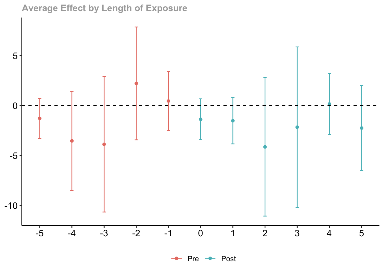
References
Callaway, Brantly, and Pedro HC Sant’Anna. 2020. “Difference-in-Differences with Multiple Time Periods.” Journal of Econometrics.